How to: Ultralytics YOLOv11 - Training Your Own AI Model

July 10, 2025

10 minutes

yolo software

Introduction.

Introducing Ultralytics YOLO11, the latest version of the acclaimed real-time object detection and image segmentation model. YOLO11 is built on cutting-edge advancements in deep learning and computer vision, offering unparalleled performance in terms of speed and accuracy. Its streamlined design makes it suitable for various applications and easily adaptable to different hardware platforms, from edge devices to cloud APIs. Read more…

Although there are abundant tutorials on how to set up YOLO and train your own model, most are very case by case and are not applicable to all users. In this post, I wanted to make a get started guide for those who may be a little lost or struggling to see where to start.

In this hands-on tutorial, you’ll discover just how easy it is to train a custom YOLOv11 model on your own image dataset. For this walkthrough, I picked a simple object—a plain eraser—and with just 7 images, achieved impressive and reliable results. If you’re new to object detection, you’ll see how quickly you can get started!

Setting up.

To start, you’ll definitely want to create a new folder to work in, and a virtual environment to isolate things. Otherwise, conflicts between packages are nearly guaranteed.

python -m venv .env

Next, activate it:

source .env/bin/activate

Now we will need the yolo11.pt pre-trained model in order to train a model of our own. To do so, you will need to select one of 5 available pre-trained models from their site. Each one has their own characteristics. For this, I will use yolo11n.pt as it is a good cross between performance and functionality.

You can read about each model and download the one that best suits you from this page (https://docs.ultralytics.com/tasks/detect)

Save the model to your working directory/folder.

The next thing to prepare ourselves will be following a specific format for our directories. Your workspace folder should look something like this:

your-project-folder/
├── images/
│   ├── train/
│   │   
│   └── val/
│      
├── labels/
│   ├── train/
│   │   
│   └── val/
│       
└── yolo11n.pt

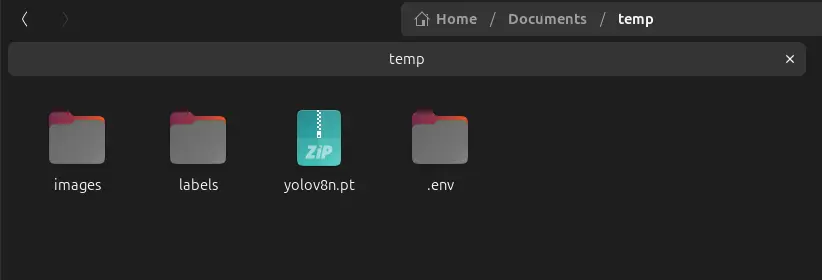
To do this, create two folders called images and labels in your root working directory respectively. Inside each of those folders, create two more subfolders, called train and val respectively. The pre-trained model you downloaded from earlier should also be in your current working directory’s root folder as shown in the diagram above.

Installing.

Now that we have an isolated environment, it is safe to install the necessary packages.

For this, we will use the python package manager, pip. From this point, I will be demonstrating how to use YOLO on a Linux machine. This should still apply to most other operating systems with minimal modifications to the commands.

Install OpenCV and Ultralytics (YOLO)

pip3 install opencv-python ultralytics

Collecting Images.

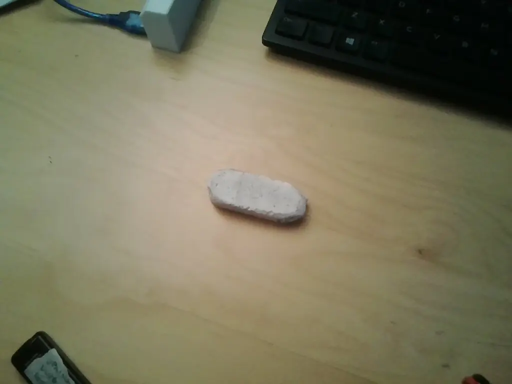
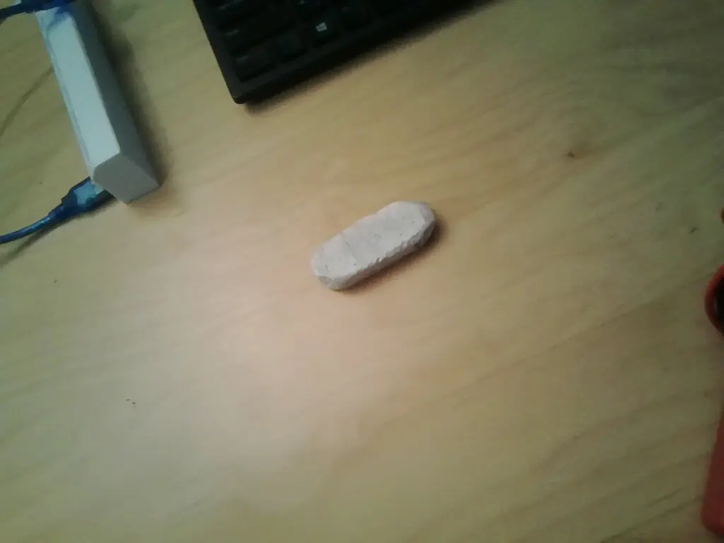
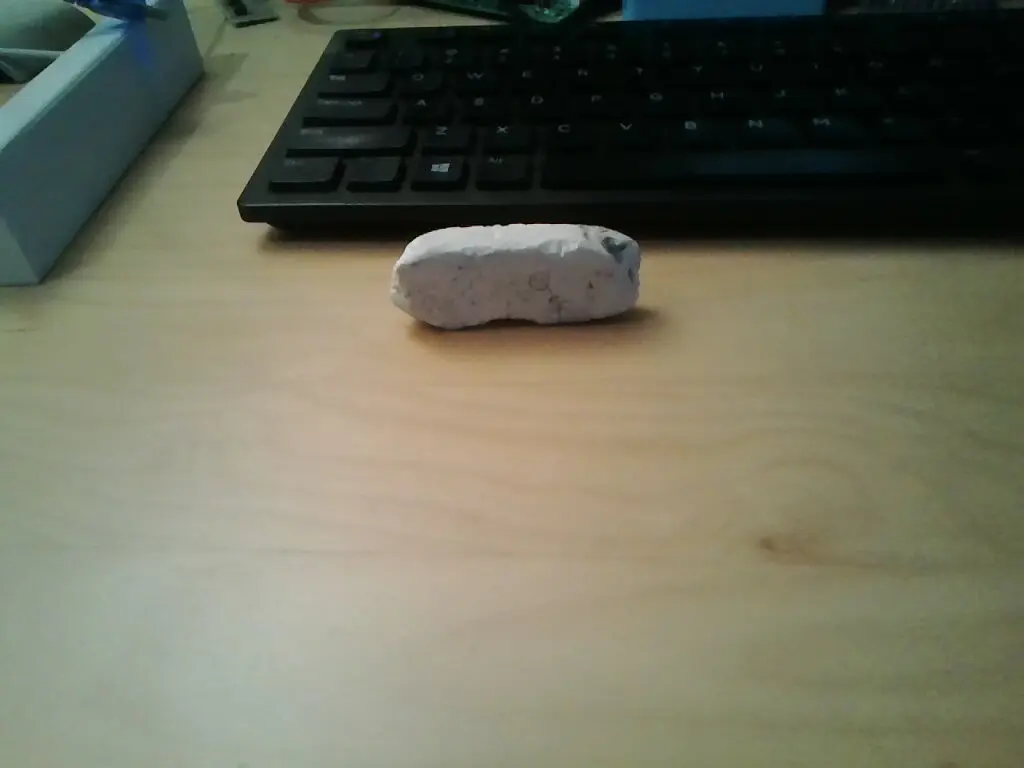
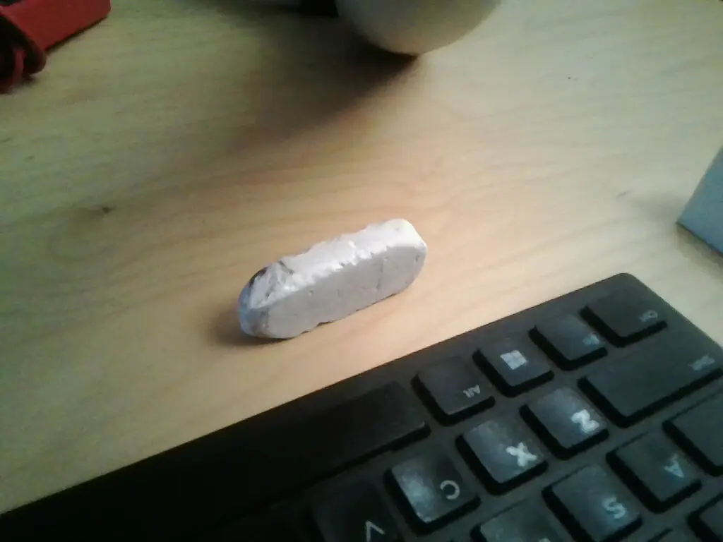
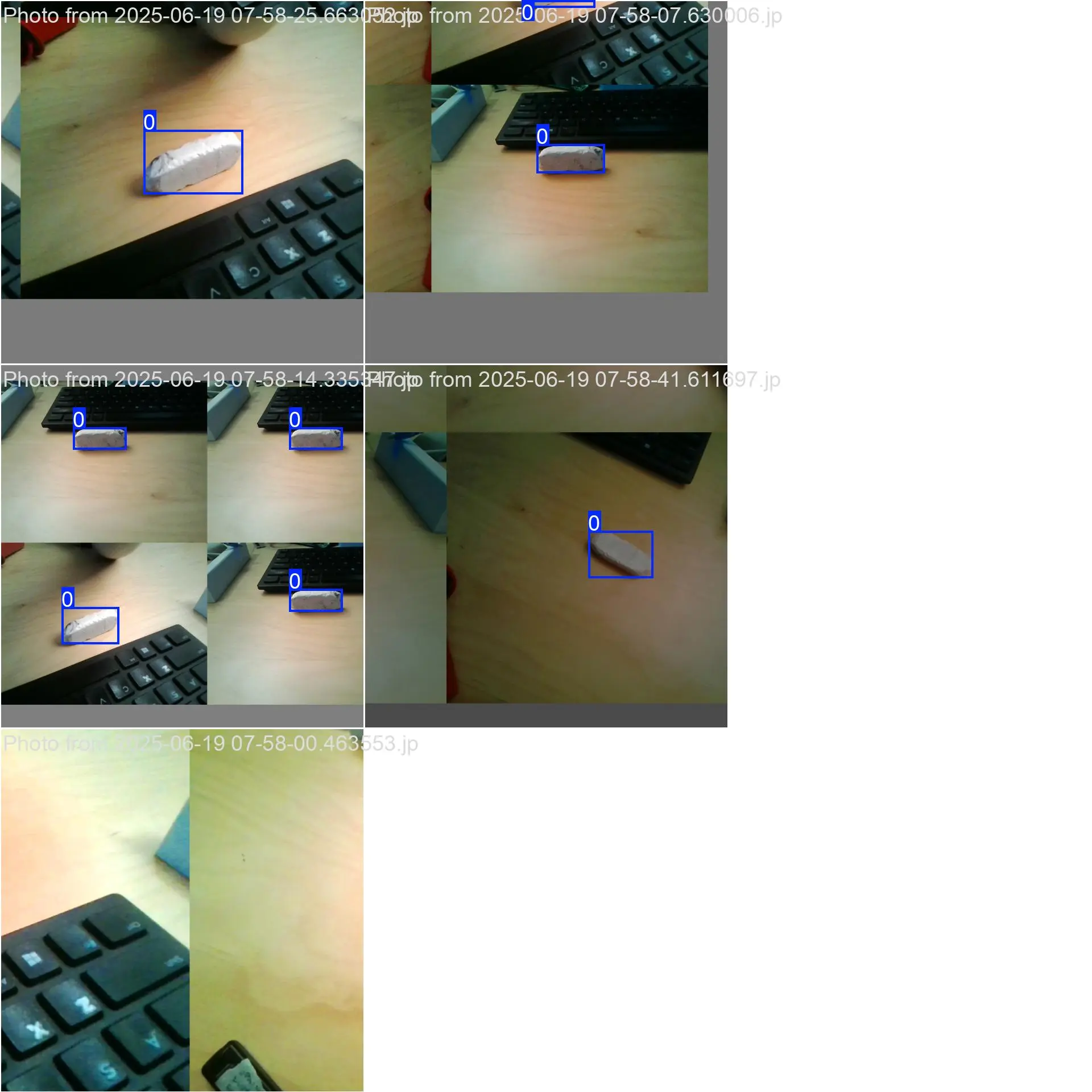
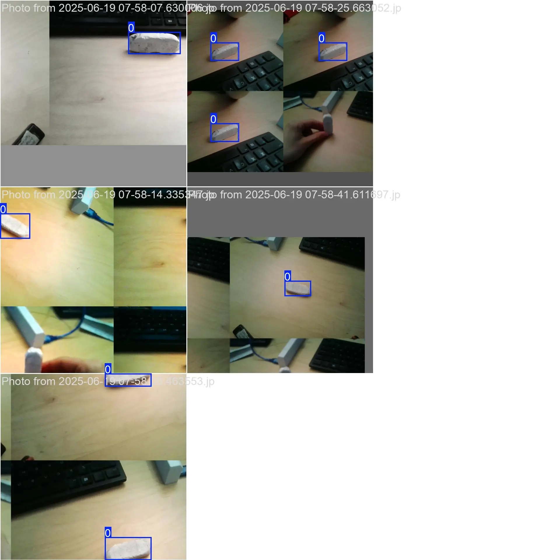
Now comes time to choose your target. If you are experimenting, you can choose a common object like I did, but if you have a specific target, use that. In order to have a versatile and robust model, you will want to photograph the object from various angles with different lighting and environments. For this demonstration, I simply used my webcam and took pictures of the eraser from different angles- not ideal but it worked out fine for this purpose.

Here are some of the ones that I used for training. Please keep in mind that these are not ideal, and using a larger dataset with lots of diversity is required to achieve best results.

If you would like to use my functional dataset, you may download it here (train/val images & train/val labels) (.zip): Download

Annotating the Images.

Now that you have collected all of your images, you must annotate them. This is the most tedious step, however that level of tediosity depends on how large your dataset is. With my small dataset with under 10 images, I was able to label and annotate in under 5 minutes.

There are numerous ways to annotate these pictures and export them in a format that appeals to the YOLO software, however I found the easiest and most efficient was to use an online tool called makesense.ai. It also supports YOLO exports which is exactly what we need.

Here’s a step-by-step process for annotating your images:

Go to makesense.ai.
Click Get Started and upload all your images that you took of your target object.
Choose Object Detection as the task type and click Start Project.
Draw bounding boxes around your target object(s) in each image.
Assign a label/class name to each bounding box (e.g., eraser).
After annotating all images, click Actions > Export annotations.
Select the YOLO format for export.
Unzip the downloaded .txt label files.

Now you have the text files. These are the annotations for each image you uploaded. Each annotation text file contains one line per object in the image, with each line following this format:

<class_id> <x_center> <y_center> <width> <height>

class_id: The numeric ID of the object class (e.g., 0 for “eraser”).
x_center and y_center: The normalized center coordinates of the bounding box (values between 0 and 1, relative to image width and height).
width and height: The normalized width and height of the bounding box (also between 0 and 1).

For example, the line:

0 0.504641 0.511757 0.198639 0.157178

means:

The object belongs to class 0 (“eraser”).
The bounding box is centered at (50.5%, 51.2%) of the image.
The bounding box covers 19.9% of the image width and 15.7% of the image height.

Assembling.

Home stretch! 🥳

Once you have the images and the annotations, you can put them into one folder. There should be an annotation with the same name for each image. If there is not, double check to make sure you didn’t lose any annotations or images anywhere along this process.

You will need to divide your assets into 2 categories known as train and val. As you may have guessed, the train assets are used to train the model, and the val assets are used to validate it. Remember the folder layout we created earlier? Well this is where that comes into play. For this to work, you will need to divide your data into 2 groups, where training is ~80% and val is ~20% of your assets.

Put 80 percent of the images into the images/train folder and their corresponding labels into the labels/train folder. Then put about 20 percent of the images into the images/val and their corresponding labels into the labels/val folder. This balance yields the best results in my experience, and is what Ultralytics and many others recommend.

your-project-folder/
├── images/
│   ├── train/
│   │   ├── img1.jpg
│   │   ├── img2.jpg
│   │   └── ...
│   └── val/
│       ├── img3.jpg
│       └── ...
├── labels/
│   ├── train/
│   │   ├── img1.txt
│   │   ├── img2.txt
│   │   └── ...
│   └── val/
│       ├── img3.txt
│       └── ...
└── yolo11n.pt

Each image in images/train has a corresponding annotation file in labels/train (e.g., img1.jpg ↔ img1.txt).
Each image in images/val has a corresponding annotation file in labels/val.
The .txt files contain the YOLO-format bounding box annotations for each image.

Once that is complete, there is only one more file to create, and then we can train the model!

Configuration.

This step is important as it tells YOLO what this data is, and where to find it.

You will need to create a .yaml file in the root of your working directory. Something easy to remember and applicable is recommended for the name. For my eraser, I named it eraser.yaml.

Put the following contents into your yaml file, and change as necessary:

train: images/train
val: images/val

nc: 1
names: ['eraser']

Here’s a quick explanation of each variable in the YAML file:

train: Specifies the path to your training dataset images.

val: Specifies the path to your validation dataset images. Example: images/val

nc: Stands for “number of classes”. Here, nc: 1 means you have one object class to detect.

names: A list of class names. Here, [’eraser’] is the only class.

This yaml format is commonly used for configuring datasets in object detection frameworks like YOLO.

Save the file.

Training Your YOLO Model.

Open your terminal in your working directory (make sure your virtual environment (.env) is activated!) and run the following command to train your model:

yolo task=detect mode=train model=yolov8n.pt data=eraser.yaml epochs=100

yolo: This is the command-line tool for running YOLO tasks.
task=detect: Specifies that you want to perform an object detection task.
mode=train: Sets the mode to training, so the model will learn from your dataset.
model=yolov11n.pt: Uses the pre-trained YOLOv8 nano model as a starting point. The .pt file is a PyTorch model checkpoint. (Change this if you downloaded a different checkpoint from earlier!)
data=eraser.yaml: Points to your dataset configuration file, which tells YOLO where to find your images and labels. (Change this to be whatever your yaml file is!)
epochs=100: Sets the number of training cycles (epochs) to 100. More epochs can lead to better accuracy, but also take longer to train. One hundred is a good balance I’ve found and works fine for most cases. Going too high can lead to a negative effect where the model loses progress. Mess around with it until you get your desired model results.

When you run this command, YOLO will start training the model using your dataset. You’ll see output in the terminal showing the training progress, including metrics like loss and accuracy. You ultimately want to see lower and lower loss as each epoch progresses, but if it fluctuates a bit, don’t worry.

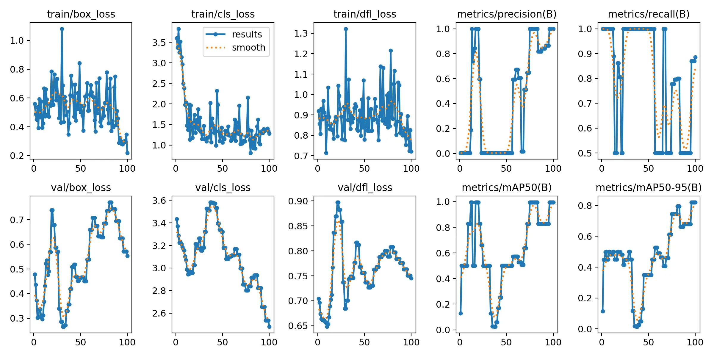
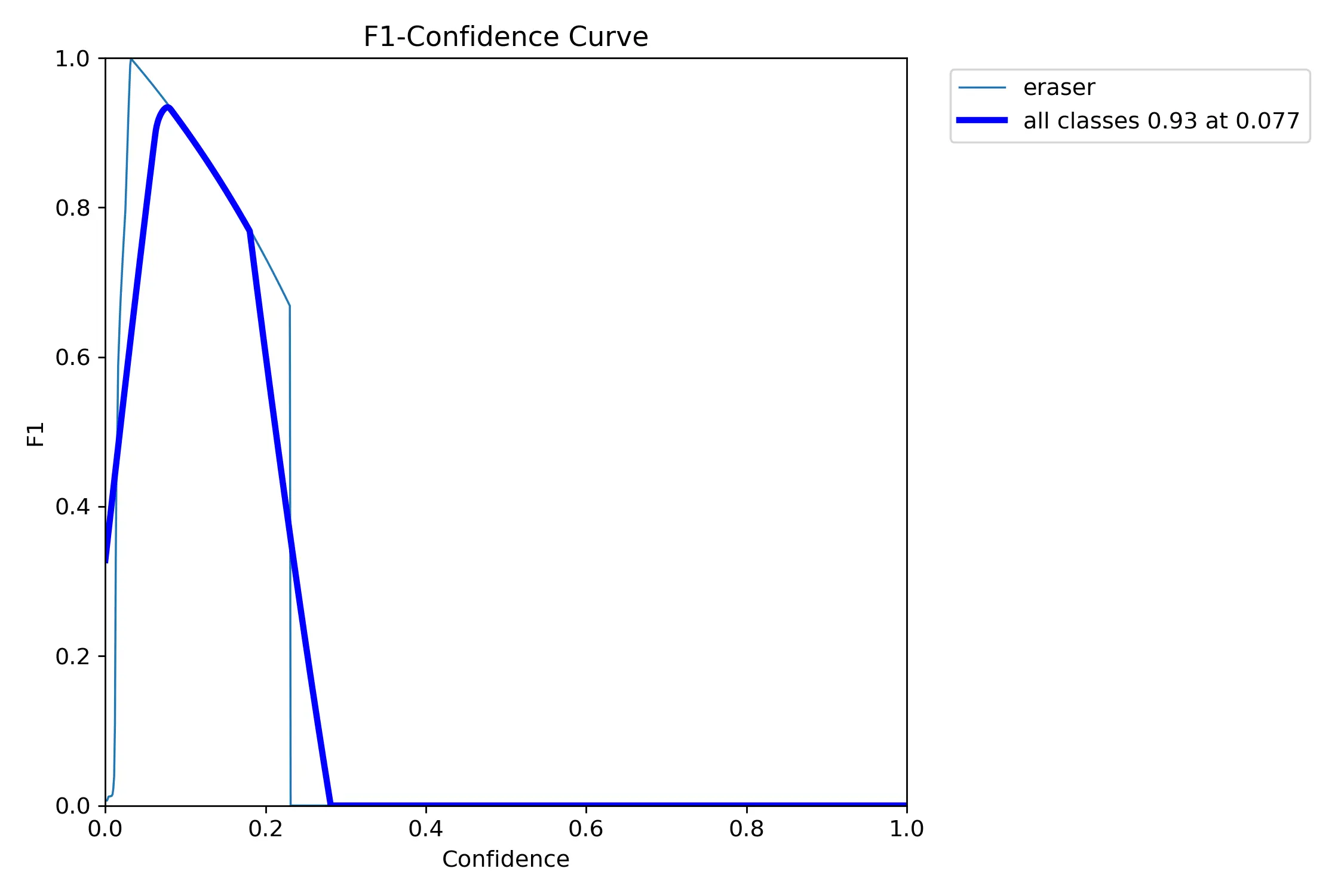
After the model finishes training, you can find the model, along with some stats on how training went in the newly created folder runs/detect/train/. There, you will find various graphs that show how the training progress went. Your model will be found under the weights folder. The best.pt model is the model you will want to use!

My results were far from perfect:

Using the Model.

You’ve done it! You have a custom trained model on your own dataset! Nice work 👏 The next step would be figuring out how on earth you use it! For this example, we will be using a webcam as our input source. So we will be able to see the model detecting our trained object(s) in real time!

In order to use the model, we will use a little bit of python, and the provided Ultralytics library (which we installed earlier).

For this, we will use the following code:

import cv2
from ultralytics import YOLO

# load the model
model = YOLO("./runs/detect/train3/weights/best.pt")  # change path if needed

# open webcam 0
cap = cv2.VideoCapture(0)

while True:
    ret, frame = cap.read()
    if not ret:
        break

    cv2.imshow("Raw Video", frame)
    key = cv2.waitKey(1)

    if key == 27:  # ESC to quit
        break

    # Run YOLO detection
    results = model(frame)[0]  # frame as input

        # plot the results on the frame
    annotated_frame = results.plot()

    cv2.imshow("Detection", annotated_frame)

cap.release()
cv2.destroyAllWindows()

Paste this into any python file. I saved mine as demo.py.

Now, from your virtual environment terminal, run the code! Make sure you are running the script with your venv activcated, otherwise you will run into errors.

python3 demo.py

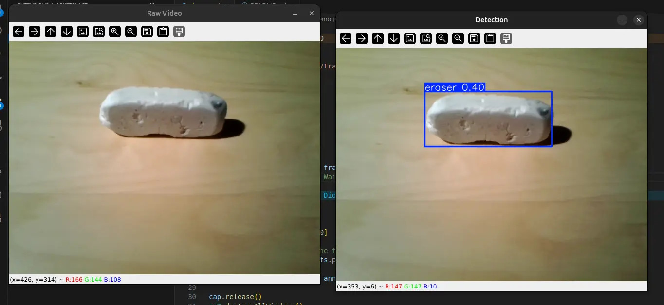
The number above the box drawn is a percentage of how convinced it is that what it is seeing is the target object. A larger number will indicate a better trained model. In my case, there were a few false positives that appeared when moving the camera around the room, which is largely due to my small dataset of 7 images that lacked diversity.

mileshilliard